Bohr model

Wednesday 6 July 2011

Bohr model

From Wikipedia, the free encyclopedia

Not to be confused with Bohr equation.

This article includes a list of references, related reading or external links, but its sources remain unclear because it lacks inline citations. Please improve this article by introducing more precise citations where appropriate. (December 2008)

The Rutherford–Bohr model of the hydrogen atom (Z = 1) or a hydrogen-like ion (Z > 1), where the negatively charged electron confined to an atomic shell encircles a small, positively charged atomic nucleus and where an electron jump between orbits is accompanied by an emitted or absorbed amount of electromagnetic energy (hν).^[1] The orbits in which the electron may travel are shown as grey circles; their radius increases as n², where n is the principal quantum number. The 3 → 2 transition depicted here produces the first line of the Balmer series, and for hydrogen (Z = 1) it results in a photon of wavelength 656 nm (red light).

In atomic physics, the Bohr model, introduced by Niels Bohr in 1913, depicts the atom as a small, positively charged nucleus surrounded by electrons that travel in circular orbits around the nucleus—similar in structure to the solar system, but with electrostatic forces providing attraction, rather than gravity. This was an improvement on the earlier cubic model (1902), the plum-pudding model (1900), the Saturnian model (1904), and the Rutherford model (1911). Since the Bohr model is a quantum physics-based modification of the Rutherford model, many sources combine the two, referring to the Rutherford–Bohr model.
The model's key success lay in explaining the Rydberg formula for the spectral emission lines of atomic hydrogen. While the Rydberg formula had been known experimentally, it did not gain a theoretical underpinning until the Bohr model was introduced. Not only did the Bohr model explain the reason for the structure of the Rydberg formula, it also provided a justification for its empirical results in terms of fundamental physical constants.
The Bohr model is a primitive model of the hydrogen atom. As a theory, it can be derived as a first-order approximation of the hydrogen atom using the broader and much more accurate quantum mechanics, and thus may be considered to be an obsolete scientific theory. However, because of its simplicity, and its correct results for selected systems (see below for application), the Bohr model is still commonly taught to introduce students to quantum mechanics, before moving on to the more accurate but more complex valence shell atom. A related model was originally proposed by Arthur Erich Haas in 1910, but was rejected. The quantum theory of the period between Planck's discovery of the quantum (1900) and the advent of a full-blown quantum mechanics (1925) is often referred to as the old quantum theory.

Origin

In the early 20th century, experiments by Ernest Rutherford established that atoms consisted of a diffuse cloud of negatively charged electrons surrounding a small, dense, positively charged nucleus. Given this experimental data, Rutherford naturally considered a planetary-model atom, the Rutherford model of 1911 – electrons orbiting a solar nucleus – however, said planetary-model atom has a technical difficulty. The laws of classical mechanics (i.e. the Larmor formula), predict that the electron will release electromagnetic radiation while orbiting a nucleus. Because the electron would lose energy, it would gradually spiral inwards, collapsing into the nucleus. This atom model is disastrous, because it predicts that all atoms are unstable.
Also, as the electron spirals inward, the emission would gradually increase in frequency as the orbit got smaller and faster. This would produce a continuous smear, in frequency, of electromagnetic radiation. However, late 19th century experiments with electric discharges through various low-pressure gases in evacuated glass tubes had shown that atoms will only emit light (that is, electromagnetic radiation) at certain discrete frequencies.
To overcome this difficulty, Niels Bohr proposed, in 1913, what is now called the Bohr model of the atom. He suggested that electrons could only have certain classical motions:

The electrons can only travel in certain orbits: at a certain discrete set of distances from the nucleus with specific energies.
The electrons of an atom revolve around the nucleus in orbits. These orbits are associated with definite energies and are also called energy shells or energy levels. Thus, the electrons do not continuously lose energy as they travel in a particular orbit. They can only gain and lose energy by jumping from one allowed orbit to another, absorbing or emitting electromagnetic radiation with a frequency ν determined by the energy difference of the levels according to the Planck relation:
$\Delta{E} = E_2-E_1=h\nu \ ,$

where h is Planck's constant.
The frequency of the radiation emitted at an orbit of period T is as it would be in classical mechanics; it is the reciprocal of the classical orbit period:
$\nu = {1\over T}$

The significance of the Bohr model is that the laws of classical mechanics apply to the motion of the electron about the nucleus only when restricted by a quantum rule. Although rule 3 is not completely well defined for small orbits, because the emission process involves two orbits with two different periods, Bohr could determine the energy spacing between levels using rule 3 and come to an exactly correct quantum rule: the angular momentum L is restricted to be an integer multiple of a fixed unit:

$L = n{h \over 2\pi} = n\hbar$

where n = 1, 2, 3, ... is called the principal quantum number, and ħ = h/2π. The lowest value of n is 1; this gives a smallest possible orbital radius of 0.0529 nm known as the Bohr radius. Once an electron is in this lowest orbit, it can get no closer to the proton. Starting from the angular momentum quantum rule Bohr^[2] was able to calculate the energies of the allowed orbits of the hydrogen atom and other hydrogen-like atoms and ions.

Electron energy levels

The Bohr model gives almost exact results only for a system where two charged points orbit each other at speeds much less than that of light. This not only includes one-electron systems such as the hydrogen atom, singly ionized helium, doubly ionized lithium, but it includes positronium and Rydberg states of any atom where one electron is far away from everything else. It can be used for K-line X-ray transition calculations if other assumptions are added (see Moseley's law below). In high energy physics, it can be used to calculate the masses of heavy quark mesons.
To calculate the orbits requires two assumptions:

Classical mechanics

The electron is held in a circular orbit by electrostatic attraction. The centripetal force is equal to the Coulomb force.

${m_e v^2\over r} = {Zk_e e^2 \over r^2}$

where m_e is the mass, e is the charge of the electron and k_e is Coulomb's constant. This determines the speed at any radius:

$v = \sqrt{ Zk_e e^2 \over m_e r}$

It also determines the total energy at any radius:

$E= {1\over 2} m_e v^2 - {Z k_e e^2 \over r} = - {Z k_e e^2 \over 2r}$

The total energy is negative and inversely proportional to r. This means that it takes energy to pull the orbiting electron away from the proton. For infinite values of r, the energy is zero, corresponding to a motionless electron infinitely far from the proton. The total energy is half the potential energy, which is true for non circular orbits too by the virial theorem.

For positronium, m_e is replaced by its reduced mass (μ = m_e/2).

Quantum rule

The angular momentum L = m_evr is an integer multiple of ħ:

$m_e v r = n \hbar$

Substituting the expression for the velocity gives an equation for r in terms of n:

$\sqrt{Zk_e e^2 m_e r} = n \hbar$

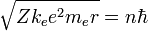
so that the allowed orbit radius at any n is:

$r_n = {n^2\hbar^2\over Zk_e e^2 m_e}$

The smallest possible value of r in the hydrogen atom is called the Bohr radius and is equal to:

$r_1 = {\hbar^2 \over k_e e^2 m_e} \approx 5.29 \times 10^{-11} \mathrm{m}$

The energy of the n-th level for any atom is determined by the radius and quantum number:

$E = -{Zk_e e^2 \over 2r_n } = - { Z^2(k_e e^2)^2 m_e \over 2\hbar^2 n^2} \approx {-13.6Z^2 \over n^2}\mathrm{eV}$

An electron in the lowest energy level of hydrogen (n = 1) therefore has about 13.6 eV less energy than a motionless electron infinitely far from the nucleus. The next energy level (n = 2) is −3.4 eV. The third (n = 3) is −1.51 eV, and so on. For larger values of n, these are also the binding energies of a highly excited atom with one electron in a large circular orbit around the rest of the atom.
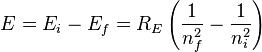
The combination of natural constants in the energy formula is called the Rydberg energy (R_E):

$R_E = { (k_e e^2)^2 m_e \over 2 \hbar^2}$

This expression is clarified by interpreting it in combinations which form more natural units:

$\, m_e c^2$ is the rest mass energy of the electron (511 keV)

$\, {k_e e^2 \over \hbar c} = \alpha \approx {1\over 137}$ is the fine structure constant

$\, R_E = {1\over 2} (m_e c^2) \alpha^2$

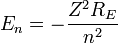
Since this derivation is with the assumption that the nucleus is orbited by one electron, we can generalize this result by letting the nucleus have a charge q = Z e where Z is the atomic number. This will now give us energy levels for hydrogenic atoms, which can serve as a rough order-of-magnitude approximation of the actual energy levels. So, for nuclei with Z protons, the energy levels are (to a rough approximation):

$E_n = -{Z^2 R_E \over n^2}$

The actual energy levels cannot be solved analytically for more than one electron (see n-body problem) because the electrons are not only affected by the nucleus but also interact with each other via the Coulomb Force.
When Z = 1/α (Z ≈ 137), the motion becomes highly relativistic, and Z² cancels the α² in R; the orbit energy begins to be comparable to rest energy. Sufficiently large nuclei, if they were stable, would reduce their charge by creating a bound electron from the vacuum, ejecting the positron to infinity. This is the theoretical phenomenon of electromagnetic charge screening which predicts a maximum nuclear charge. Emission of such positrons has been observed in the collisions of heavy ions to create temporary super-heavy nuclei.^{[citation needed]}
The Bohr formula properly uses the reduced mass of electron and proton in all situations, instead of the mass of the electron: $m_\text{red} = \frac{m_e m_p}{m_e + m_p} = m_e \frac{1}{1+m_e/m_p}$ . However, these numbers are very nearly the same, due to the much larger mass of the proton, about 1836.1 times the mass of the electron, so that the reduced mass in the system is the mass of the electron multiplied by the constant 1836.1/(1+1836.1) = 0.99946. This fact was historically important in convincing Rutherford of the importance of Bohr's model, for it explained the fact that the frequencies of lines in the spectra for singly ionized helium do not differ from those of hydrogen by a factor of exactly 4, but rather by 4 times the ratio of the reduced mass for the hydrogen vs. the helium systems, which was much closer to the experimental ratio than exactly 4.0.
For positronium, the formula uses the reduced mass also, but in this case, it is exactly the electron mass divided by 2. For any value of the radius, the electron and the positron are each moving at half the speed around their common center of mass, and each has only one fourth the kinetic energy. The total kinetic energy is half what it would be for a single electron moving around a heavy nucleus.

$E_n = {R_E \over 2 n^2 }$ (positronium)

Rydberg formula

The Rydberg formula, which was known empirically before Bohr's formula, is now in Bohr's theory seen as describing the energies of transitions or quantum jumps between one orbital energy level, and another. Bohr's formula gives the numerical value of the already-known and measured Rydberg's constant, but now in terms of more fundamental constants of nature, including the electron's charge and Planck's constant.
When the electron gets moved from its original energy level to a higher one, it then jumps back each level till it comes to the original position, which results in a photon being emitted. Using the derived formula for the different 'energy' levels of hydrogen one may determine the 'wavelengths' of light that a hydrogen atom can emit.
The energy of a photon emitted by a hydrogen atom is given by the difference of two hydrogen energy levels:

$E=E_i-E_f=R_E \left( \frac{1}{n_{f}^2} - \frac{1}{n_{i}^2} \right) \,$

where n_f is the final energy level, and n_i is the initial energy level.
Since the energy of a photon is

$E=\frac{hc}{\lambda}, \,$

the wavelength of the photon given off is given by

$\frac{1}{\lambda}=R \left( \frac{1}{n_{f}^2} - \frac{1}{n_{i}^2} \right). \,$

This is known as the Rydberg formula, and the Rydberg constant R is

R E / h c

, or

R E / 2π

in natural units. This formula was known in the nineteenth century to scientists studying spectroscopy, but there was no theoretical explanation for this form or a theoretical prediction for the value of R, until Bohr. In fact, Bohr's derivation of the Rydberg constant, as well as the concomitant agreement of Bohr's formula with experimentally observed spectral lines of the Lyman (

n f = 1

), Balmer (

n f = 2

), and Paschen (

n f = 3

) series, and successful theoretical prediction of other lines not yet observed, was one reason that his model was immediately accepted.
To apply to atoms with more than one electron, the Rydberg formula can be modified by replacing "Z" with "Z - b" or "n" with "n - b" where b is constant representing a screening effect due to the inner-shell and other electrons (see Electron shell and the later discussion of the "Shell Model of the Atom" below). This was established empirically before Bohr presented his model.

Moseley's law and calculation of K-alpha X-ray emission lines

Niels Bohr said in 1962, "You see actually the Rutherford work [the nuclear atom] was not taken seriously. We cannot understand today, but it was not taken seriously at all. There was no mention of it any place. The great change came from Moseley."
In 1913 Henry Moseley found an empirical relationship between the strongest X-ray line emitted by atoms under electron bombardment (then known as the K-alpha line), and their atomic number Z. Moseley's empiric formula was found to be derivable from Rydberg and Bohr's formula (Moseley actually mentions only Ernest Rutherford and Antonius Van den Broek in terms of models). The two additional assumptions that [1] this X-ray line came from a transition between energy levels with quantum numbers 1 and 2, and [2], that the atomic number Z when used in the formula for atoms heavier than hydrogen, should be diminished by 1, to (Z-1)².
Moseley wrote to Bohr, puzzled about his results, but Bohr was not able to help. At that time, he thought that the postulated innermost "K" shell of electrons should have at least four electrons, not the two which would have neatly explained the result. So Moseley published his results without a theoretical explanation.
Later, people realized that the effect was caused by charge screening, with an inner shell containing only 2 electrons. In the experiment, one of the innermost electrons in the atom is knocked out, leaving a vacancy in the lowest Bohr orbit, which contains a single remaining electron. This vacancy is then filled by an electron from the next orbit, which has n=2. But the n=2 electrons see an effective charge of Z-1, which is the value appropriate for the charge of the nucleus, when a single electron remains in the lowest Bohr orbit to screen the nuclear charge +Z, and lower it by -1 (due to the electron's negative charge screening the nuclear positive charge). The energy gained by an electron dropping from the second shell to the first gives Moseley's law for K-alpha lines:

$E= h\nu = E_i-E_f=R_E (Z-1)^2 \left( \frac{1}{1^2} - \frac{1}{2^2} \right) \,$

$f = \nu = R_v \left( \frac{3}{4}\right) (Z-1)^2 = (2.46 \times 10^{15} \operatorname{Hz})(Z-1)^2.$

Here, R_v = R_E/h is the Rydberg constant, in terms of frequency equal to 3.28 x 10¹⁵ Hz. For values of Z between 11 and 31 this latter relationship had been empirically derived by Moseley, in a simple (linear) plot of the square root of X-ray frequency against atomic number (however, for silver, Z = 47, the experimentally obtained screening term should be replaced by 0.4). Notwithstanding its restricted validity^[3] did Moseley's law not only establish the objective meaning of atomic number (see Henry Moseley for detail) but, as Bohr noted, it also did more than the Rydberg derivation to establish the validity of the Rutherford/Van den Broek/Bohr nuclear model of the atom, with atomic number as nuclear charge.
The K-alpha line of Moseley's time is now known to be a pair of close lines, written as (K_α1 and K_α2) in Siegbahn notation.

Refinements

It has been suggested that this article or section be merged with Bohr–Sommerfeld theory. (Discuss) Proposed since March 2009.

Elliptical orbits with the same energy and quantized angular momentum

Several enhancements to the Bohr model were proposed; most notably the Sommerfeld model or Bohr-Sommerfeld model, which suggested that electrons travel in elliptical orbits around a nucleus instead of the Bohr model's circular orbits.^[1] This model supplemented the quantized angular momentum condition of the Bohr model with an additional radial quantization condition, the Sommerfeld-Wilson quantization condition^[4]^[5]

$\int_0^T p_r \,dq_r = n h \,$

where p_r is the radial momentum canonically conjugate to the coordinate q which is the radial position and T is one full orbital period. The integral is the action of action-angle coordinates. This condition, suggested by the correspondence principle, is the only one possible, since the quantum numbers are adiabatic invariants.
The Bohr-Sommerfeld model was fundamentally inconsistent and led to many paradoxes. The magnetic quantum number measured the tilt of the orbital plane relative to the xy-plane, and it could only take a few discrete values. This contradicted the obvious fact that an atom could be turned this way and that relative to the coordinates without restriction. The Sommerfeld quantization can be performed in different canonical coordinates, and sometimes gives answers which are different. The incorporation of radiation corrections was difficult, because it required finding action-angle coordinates for a combined radiation/atom system, which is difficult when the radiation is allowed to escape. The whole theory did not extend to non-integrable motions, which meant that many systems could not be treated even in principle. In the end, the model was replaced by the modern quantum mechanical treatment of the hydrogen atom, which was first given by Wolfgang Pauli in 1925, using Heisenberg's matrix mechanics. The current picture of the hydrogen atom is based on the atomic orbitals of wave mechanics which Erwin Schrödinger developed in 1926.